
< Previous lab day | Module 3 lab index | Next lab day >
Introduction
Today you will start collecting the key data for your chondrocyte or stem cell phenotype experiment. Recall that chondrocytes may de-differentiate to fibroblasts if not kept in the appropriate environment. So, how do we tell chondrocytic and non-chondrocytic cell types apart?
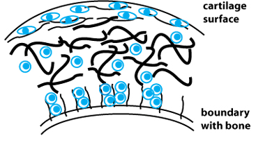
Schematic of cartilage tissue. Collagen fibers are shown in black, chondrocytes in light blue. Collagen fiber thickness and orientatiom, along with chondrocyte density and morphology, vary with the tissue depth. Adapted from: V. C. Mow, A. Ratcliffe, and S. L. Y. Woo, eds. Biomechanics of Diarthrodial Joints. Vol. 1, Chapter 8. New York, NY: Springer-Verlag, 1990. ISBN: 9780387973784.
Folks trying to engineer cartilage tissue have been in interested in this and similar questions for some time. After all, the more closely an in vitro or in vivo model construct can mimic natural tissue and promote its development, the more successful it may be for wound and disease repair. Engineering tissue thus requires an expert understanding of what the native tissue is like. Articular cartilage is a water-swollen protein network consisting of >50% collagen Type II, along with small amounts of collagen Types IX and XI. The collagen fibrils vary in diameter, cross-linking density, and orientation (random or aligned) depending on the depth of the tissue cross-section that is examined (see figure). Unlike cartilage, many other connective tissues are composed primarily of collagen Type I.
Extracellular matrix (ECM) proteins such as the collagens must be synthesized by cells. Chondrocytes readily synthesize collagen II, while fibroblasts and mesenchymal stem cells primarily synthesize collagen I. Thus, the expression and production of different collagens is one way to distinguish these cells types. To study collagen at the gene transcript level, you will break open and homogenize your cells using a lysis reagent and column (QIAshredder) and then isolate RNA using an RNeasy kit from Qiagen. The RNeasy kit includes silica gel columns, similar to the ones you used to purify DNA in Module 1, that selectively bind RNA (but not DNA) that is >200 bp long under appropriate buffer conditions. Due to size exclusion, the resultant RNA is somewhat enriched in mRNAs relative to rRNA and tRNA. To further purify for mRNA, one could use a polyT affinity column to capture the polyA tail of this RNA type, but we will not do this today.
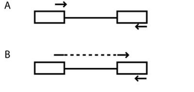
Schematic of primer design for RT-PCR. Boxes and lines represent exons and introns, respectively. Arrows represent primers. (A) Each primer anneals to a sequence from only one exon. (B) The top primer spans two exons, thus reducing or eliminating product contamination by genomic DNA. (The dashed line indicates that the surrounding solid lines constitutes one continuous primer.)
After eluting and measuring your total RNA, you will perform RT-PCR to turn the mRNA into cDNA and amplify the gene transcripts of interest, namely those for the collagen I and collagen II alpha chains. We will use the same 1-step RT-PCR kit from Qiagen that we used in Module 1. For RT-PCR, primer design must be appropriate for a cDNA rather than genomic DNA. For example, a single primer that includes sequence from two neighbouring exons (along with a second primer that has sequence from just one exon) will amplify mRNA but not genomic DNA, which may be present as a contaminant (see also figure). What will happen if each primer contains sequence from only one exon?
Next time you will run the amplified cDNA products out on an agarose gel, and compare the collagen II:I ratios for your two culture conditions. (Recall that a high ratio indicates a more chondrocyte-like phenotype.) As you may have noticed by now, agarose gels do not have a large dynamic range. In an ideal world (perhaps a future iteration of this module!), we would want to use a more sensitive method for quantifying the transcripts. To get more quantitative and reliable results, one can use real-time-PCR, sometimes called RT-PCR, confusingly! The method is also called q-PCR, for quantitative-PCR. In q-PCR, the amount of DNA (often a cDNA, as in RT-PCR) is measured after each cycle of PCR. This assay is done by using a dye that fluoresces only when it binds to DNA (similar to ethidium bromide staining), or even a tagged primer that fluoresces only when it binds to the desired product. Several of the fluorophores available exploit FRET (fluorescence resonance energy transfer) between two molecules. As the DNA is amplified, fluorescence is repeatedly measured and increases exponentially over time. Finally, cDNA product renaturing competes with primer annealing and the fluorescence intensity plateaus rather than growing. Comparisons between samples are done using data in the exponential regime.
Data analysis for q-PCR can be complicated, and we won't go into all the details in this course. However, even for end-point RT-PCR, one semi-quantitative technique that can be used to compare transcripts from different samples is normalization with a housekeeping gene. That is, one simultaneously amplifies the cDNA of interest and a cDNA for a protein such as GAPDH. This approach is similar to running a loading control on a gel, but trickier! The primers for the two genes must be compatible – e.g., they must not hybridize with each other. Moreover, the primer amount must be carefully optimized such that the housekeeping gene (high abundance) isn't totally saturated when the gene of interest (often low abundance) isn't even readable on the gel. Finally, ideally the housekeeping gene should have a similar amplification efficiency to the gene of interest. Today we will use primers for GAPDH as a control, at two different optimized concentrations for the two different collagen primer sets.
Next time (day 5) we'll initiate an assay called ELISA to observe collagen at the protein (rather than transcript) level and also begin analysis of the data collected thus far.
Protocols
If you got to go to the Tissue Culture first on Day 2, you will go in the second cohort today (and vice-versa). If you are in the second group, use the time that you are waiting to prepare your RNase-free area, label tubes that you will need, etc.
Part 1: Prepare Cell Lysates
You will prepare cell-bead samples in two different ways: one will allow you to count your cells, and is suitable for RNA preparation, while the other one will involve a more stringent bead/matrix dissolution for better protein recovery. Remember to label your samples carefully at every step.
- Before proceeding, briefly observe the cell-bead constructs under the microscope - what is the cell morphology and density like in each sample?
- Let the teaching faculty know if you have difficulty focusing within a bead.
- Aspirate the culture medium from each of your samples. Be careful not to suck up the beads, while using a serological pipet just as you did when washing your freshly synthesized beads. A 10 mL pipet size should work well for most beads, while for very delicate beads, you should use a 2 mL serological pipet or even a P1000.
- About half of your beads will be used to measure protein content: move these to an eppendorf tube. The goal is about 10-15 (2-3 mm) beads per tube.
- For large beads (4-5 mm), you might use only 5-10 beads, and for very small beads (<1 mm), you might use 20 or more.
- The other half will be used to isolate RNA. Using a sterile spatula, transfer the beads into a fresh well of your 6-well plate. This transfer step is to exclude any cells that are growing on the bottom of the plate (as opposed to actually in the beads) from analysis.
Samples for RNA
- Rinse the transferred bead-cell constructs with 4 mL of warm PBS, then aspirate the buffer.
- Add 3 mL of EDTA-citrate buffer, and incubate at 37 °C for 10 min.
- Meanwhile, prepare the beads for the protein assay as described below.
- Now recover your cells:
- Add 3 mL of warm complete culture medium, pipet up and down to break up the beads (you may find this easier with a 1 mL pipetman rather than a serological pipet), and transfer to a 15 mL conical tube.
- Spin the cells down at 1900g for 6 min (using the centrifuge that is in the TC room).
- Resuspend in ~ 1-1.5 mL of culture medium, and write down what you use. Mix thoroughly by pipetting, then set aside a 90 μL aliquot of your cells for counting, and put the rest of the cells into another eppendorf tube.
- While one of you begins the spin in the main lab (see Part 2), the other should count your cell aliquot as on Day 2, at a 9:1 ratio with Trypan blue. Separately calculate the approximate numbers of live and of dead cells.
- Recall that you must multiply by 10,000 (and your dilution factor) to convert a cell count to a cells/mL concentration.
Samples for Protein
- Per eppendorf tube (typically 10-15 beads), add 133 μL of EDTA-citrate buffer, and pipet up and down for 20-30 seconds to dissolve the beads. The resulting solution may be viscous.
- Pipet 33 μL of 0.25 M acetic acid into each eppendorf tube.
- Finally, pipet 33 μL of 1 mg/mL pepsin in 50 mM acetic acid into each tube and mix well.
- Move your eppendorf tubes into the rack in the 4 °C fridge. Tomorrow we will move them to the freezer.
Part 2: RNA Isolation and Measurement
- Pellet the cells for RNA isolation back in the main lab (10 min at 500 g).
- Before pelleting your cells, clean your microfuge. You can finish setting up your RNA work area while the cells spin down. See Module 1 Day 3 if you need a refresher.
- Remove the supernatant from your cell pellets using pipet tips from an RNase free tip box. (Discard this and other supernatants in a conical waste tube.)
- Now, in the fume hood, add 350 μL RLT with β-mercaptoethanol to each cell sample – vortex or pipet to mix.
- If you have more than 5 million cells, you will need to double the amount of RLT used - talk to the teaching faculty.
- Add each cell lysate to a separate QIAshredder column, which is used to remove particulate matter. Microfuge the columns (over a 2 mL collection tube) for 2 min at max speed.
- Add 1 volume (slightly > 350 μL) of 70% ethanol to each lysate and pipet to mix.
- Apply each sample (including any precipitate) to a separate RNeasy mini column (over a tube). Microfuge for 15 sec and discard the flowthrough.
- Add 700 μL RW1 buffer to each column. Microfuge 15 sec and discard the eluant again.
- Transfer the columns to fresh 2 mL collection tubes. Then add 500 μL RPE buffer atop the columns, microfuge as before (15 sec), and discard the flowthrough.
- Repeat the addition of 500 μL RPE, but this time centrifuge for 2 min. prior to discarding the flowthrough.
- Centrifuge the column/tube "dry" for 1 min. Running a column like this helps to fully dry it, and to prevent carryover of ethanol.
- Trim the caps off of two new 1.5 ml eppendorf tubes (save the caps!) and label the sides of the tubes.
- Transfer the dried columns into the trimmed eppendorf tubes and elute the RNA from the columns by adding 50 μL of RNase-free water to each. Microfuge for 1 min then cap the tubes and store the eluants on ice.
- Measure the concentration of your RNA samples as you did in Module 1, but using a somewhat higher concentration (5 μL RNA in 495 μL water). Remember to take a measurement at both 260 and 280 nm, using wavelength scan mode.
- You will use slightly different cuvettes than in Module 1. For your blank and samples, make sure the cuvettes are always oriented the same way (for example, with the "eppendorf" label always on the left-hand side).
- Note the RNA concentrations of your samples in the table below, using the fact that 40 μg/mL of RNA will give a reading of A260 = 1.
- Ideally, you will use 100 ng of RNA in each RT-PCR reaction. However, you also want all reactions to start with an equal amount of RNA template. Because you are doing two reactions per RNA sample, at most you can use 20 μL of template per reaction. If you can use 100 ng per reaction within these contraints, do so. Otherwise, figure out which one of your samples is limiting, and scale all the other sample amounts that you add so they are equal. The table below may be helpful.
- Finally, note that your RNA should be diluted in water such that you add 30 μL of template per RT-PCR reaction.
| SAMPLE | A260 | RNA CONC. μg/mL) | MAX RNA PER RXN (ng in 20 μL) | VOLUME RNA NEEDED PER RXN | VOLUME WATER NEEDED PER RXN |
|---|---|---|---|---|---|
| 1 | |||||
| 2 |
Part 3: RT-PCR
- The thermal cycler will be preheated to 50 °C while you prepare your samples. This is required for the procedure to work optimally.
- Set up your reactions on a cold block as usual. You will prepare two reactions for each of your samples: one to amplify collagen I, and one for collagen II.
- From one of the shared stocks, pipet 20 μL of Master Mix I into each of two well-labeled PCR tubes, and 20 μL of Master Mix II into two more. The Master mixes contain water, buffer, dNTPS, primers, and and an enzyme mixture.
- For the collagen I reaction: collagen I primers are at 0.3 μM, and GAPDH primers are at 0.1 μM.
- For the collagen II reaction: collagen II primers are at 0.1 μM, and GAPDH primers are at 0.6 μM.
- Prepare your diluted RNA templates according to the calculations you performed in Part 2. You should make a little more than 60 μL of each sample, so you don't run out due to pipetting errors.
- Now you can add 30 μL of the appropriate RNA to each tube containing Master Mix. Be sure to do one collagen I and one collagen II reaction for each sample.
- The following thermal cycler program will be used:
| SEGMENT | CYCLES | TEMPERATURE (° C) | TIME | PURPOSE |
|---|---|---|---|---|
| 1 | 1 | 50 | 30 min | reverse transcription |
| 2 | 1 | 95 | 15 min | activate polymerase, deactivate RT enzymes, denature template |
| 3 | 30 | 94 | 1 min | denature (PCR) |
| 54 | 1 min | anneal (PCR) | ||
| 72 | 1 min | extend (PCR) | ||
| 4 | 1 | 72 | 10 min | final extension |
After the RT-PCR is completed, the teaching faculty will store the samples in the freezer until next time.
In whatever time remains today, you can continue discussion of your shared research idea with your partner, work on your Module 3 report, etc.
For Next Time
- Write a brief response (250 ± 50 words) to one of the excerpts that were handed out in lecture and lab.
- These excerpts are drawn (with some editing) from previous 20.109 student essays about the prospect of standardization in tissue engineering.
- You may revise the response you started during lecture, or write a brand new one.
Reagent List
- Culture medium as on Day 1
- Release Buffer for Beads
- 150 mM NaCl
- 55 mM sodium citrate
- 30 mM EDTA
- For protein extraction
- 0.25 M acetic acid
- pepsin (Sigma), at 1 mg/mL in 50 mM acetic acid
- note: in future years, a follow-up treatment should be done with elastase to improve extraction; rather, breakdown of polymeric to monomeric collagen (piloted summer 2010, see TA notes)
- For RNA extraction
- Qiagen QIAshredder columns
- Qiagen RNeasy kit
- RLT needs to have βmercaptoethanol added before use (just an aliquot, stable for 1 month)
- buffer PE needs to have ethanol added prior to first use
- RT-PCR Master Mixes
- using 1-step RT-PCR kit from Qiagen
| COMPONENET | CONCENTRATION | VOLUME |
|---|---|---|
| Primers | variable: 0.1, 0.3, or 0.6 μM | 1.5 μL of 1:5 dilution each |
| dNTPs | 400 μM each | 2 μL |
| Enzymes | unknown | 2 μL |
| Reaction buffer | N/A (multi-component) | 10 μL |
| Water | N/A | 3 μL |
| Template (+ more water) | 1 pg - 2 μg | Added by students |
- Primers
- CN I forward; reverse [~200 bp]: CGAGGTCGCACTGGTGATG ; ATGTTCTCGATCTGCTGGCT
- CN II forward; reverse [~400 bp]: CTGGCTCCCAACACCGCCAACGTC ; TCCTTTGGGTTTGCAATGGATTGT
- G3PDH forward; reverse [~100 bp]: ATCAAGAAGGTGGTGAAGCAGG ; TGAGTGTCGCTGTTGAAGTCG