
Back to Newton's method: It turns out that the end result (the point to which the method converges, if any) is strongly dependent on the initial guess. Furthermore, the dependence on the first guess can be rather surprising. The set of points that converge to a given root is called the basin of attraction of that root (for the iteration under discussion). I would like us to visualize the basins of attraction by coloring each starting point with a color that corresponds to the root it converges to. The different basins will thus be given different colors.
With MATLAB® we can easily visualize which solution is chosen as a function of the initial guess. While this can be done for 1D, we will do it for 2D and learn how to do some simple linear algebra at the same time.
Generalizing Newton's method for higher dimensions is actually quite straightforward: Instead of one function \(f\), we have many, written as a vector \(\vec f\), and instead of one independent variable (\(x\)) we have many, again, written as a vector, \(\vec x\). Thus we are looking for the vector \(x\) for which:
\begin{equation} \label{eq:4} \vec f(\vec x)=\vec 0 \end{equation}
The update rule is slightly different since derivatives are more complicated in higher dimensions:
\begin{equation} \label{eq:newtons:multi:d} \vec x_{n+1}=\vec x_n- (J\vec f)^{-1} \vec f(\vec x_n). \end{equation}
Here \(Jf\) is the Jacobian matrix of \(\vec f\), that is a matrix whose term in the \(i-\)th row and \(j-\)th column is
\begin{equation} \label{eq:5} (J\vec f)_{ij}=\frac{\partial f_i}{\partial x_j}. \end{equation}
Notice that the Jacobian depends on \(\vec x\) and thus needs to be re-evaluated at every step (just like the derivative in one-dimensional Newton's method). The two parts in the right-most term of (2) are multiplied together in the linear algebra sense of the word. The power \(-1\) is matrix inverse (and not multiplicative inverse) and thus another way of writing the update rule is
\begin{equation} \label{eq:6} (J\vec f) \delta\vec x_n= (J\vec f) (\vec x_{n+1}-\vec x_n)=-\vec f(\vec x_n). \end{equation}
This formulation is a much better way of understanding Newton's method, as it exposes what is going on: The approximation is updated so that if the linear approximation to \(\vec f\) (given by the Jacobian matrix) were exact, the approximation would equal the exact root in one step.
How to implement? First we need a specific function: \(\vec f([x,y]^t)=[x^3-y,y^3-x]^t\) and thus the Jacobian matrix is \((\begin{smallmatrix} 3x^2 & -1 \\ -1& 3y^2 \end{smallmatrix})\). In MATLAB we want to have one variable, say \(X\), be a column vector that holds both \(x\) and \(y\). The code for a simple Newton method for \(f\) would be:
X=[1;2]; % the starting point. Notice the use of semicolon to define a column vector for j=1:10% iterate 10 times% let's do this using variables so that we can see what's going on:f=[X(1)^3 - X(2), X(2)^3 - X(1)]';% Another way to define a% column vector is to define a row% vector and then transpose it using% the apostrophe '. WARNING the [ ]% is a prime example of how matlab% can try to be too smart: look at% the difference between% [1+2,3]% [1 +2,3] and% [1 + 2 , 3] all legal% expressions, but one gives an% unexpected answer since we can use% space instead of comma to separate% terms in a row vector.Jf=[3*X(1)^2, -1; -1, 3*X(2)^2];% the Jacobian matrix. Notice the % semicolon after the second% term. This is like saying "now % start a new row".X=X-Jf\f;% the update rule. This does not invert the% matrix. By using "left divide" the linear system is solved,% this is equivalent but faster than inverting and multiplyingendformat long% to see the full precisionX % so that we see the final answer format short% to only see 4 digits again
Exercise 11. Multi-dimensional Newton's method
-
What are the 3 roots of \(\vec f\) in the code above? (think of them as
r1,r2,r3.) - Implement the program above and play around with the starting point to get several different answers. If you get a warning about singular matrices, don't worry about it.
-
Find the Jacobian matrix, \(J\vec g\), of:
\begin{equation*} \vec g(\vec x)= \begin{pmatrix} \sin(x_1+2x_2^2)-x_2\\ x_1^2x_2-x_1 \end{pmatrix} \end{equation*}
- The function \(g\) has many roots; modify the Newton solver to find some them by manually starting at different places.
- Are you iterating enough times? Check that the results you get are a good enough root, and if they are not, change the number of iterations so that they are.
Now here's the run-up to the next project: We want to plot the "basin of attraction" of each of the three zeros (what are they?) of the function \(\vec f\) (not \(\vec g\)). This will be your first project, but first we need to discuss how to plot the result. For an initial point \(X_0\) we can run the Newton code and after several iterations (10 in the example above) it will arrive near (in most cases) one of three roots, say \(r_1, r_2, r_3\). To visualize the basin of attraction, we go over a grid of points \(X_0\) and color them according to the to the specific zero the Newton's method algorithm ends up being close to after starting from \(X_0\). If the algorithm is not close to any of them, we put a fourth color. While it is true that normally we do not know what the zeros are, but this is also interesting in the case that we do know what they are, so we are using the a priori information about the location of the roots in order to visualize the basin of attraction.
To do this we need if-else-end statements:
if norm(X-r1)<1e-8 % if the distance between X and r1 is less than 10^-8 c='r'; % use the color red elseif norm(X-r2)<1e-8 c='b'; % use the color blue elseif norm(X-r3)<1e-8 c='g'; % use the color green else % if not close to any of the roots c='k'; % use the color black end plot(x,y,'.','color',c);% plot a point at X_0, (not the final point X!)% with the color c
Project 1. Place the Newton code, and the if-then-else code above inside two nested for loops, looping over \(x-\) values and \(y-\) values from -2 to 2 (perhaps with a small step-size of 0.1 or 0.01). For each iteration set the starting point to [x,y]' before the Newton's Method part, and then plot the color point corresponding to the location of the resulting zero. So that the subsequent plot commands do not erase the previous ones, put:
clf% clear the current Figure hold on% make sure subsequent plots do not erase the previous ones.
before the for loops. Thus the pseudo-code for this construction is:
initialize figure for x values for y values let X0=(x,y) be the starting point for Newton's method find the color corresponding to the final point of iteration X plot point X0 with correct color end loop y end loop xIf this is your first programming project, you might get frustrated at how difficult it seems to get everything in place. There's no way around it. Read you own code carefully. Give good names to your variables. Try to explain the code to someone else.
That said, there are several hints I can give:
| Hint 1. | If MATLAB is stuck, use Ctrl C to abort from a long calculation or to reset the command line. |
| Hint 2. | If MATLAB is spewing out too much onto the screen and you cannot see what you want to see, add semi-colons (;) to the end of the "offending" lines to prevent MATLAB from doing that. |
| Hint 3. | If all the points seem to be plotted at the roots rather than at the original points, you are probably using \(X\) to do the plotting rather than the original point (x,y) from the loop. |
| Hint 4. | If you are getting warnings from MATLAB that your "Matrix is close to singular or badly scaled" don't worry about it too much. It means that your algorithm has passed through a point where the Jacobian matrix is singular. The result from that point is unreliable, but there should be (relatively) few of these points, and so the overall picture will be preserved. |
| Hint 5. | If you always only have one point on your plot, you are probably not holding the plot properly. The two lines of code under the description of the project should be before the for loops (and not anywhere else). |
| Hint 6. | What is the solution supposed to look like? My result can be seen in Fig. 1. Increasing the number of iterations should make the black regions (places that have not converged) smaller. |
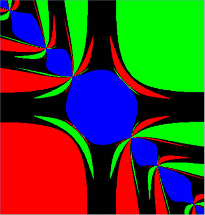
Figure 1. Basin of attraction for \(f([x,y]^t)=(x^3-y,y^3-x)^t\).