
1.8.1 Adams-Bashforth Methods
Measurable Outcome 1.15, Measurable Outcome 1.17, Measurable Outcome 1.18, Measurable Outcome 1.19
Adams-Bashforth methods are explicit methods of the form,
Thus, the basic time derivative approximation remains the same for all \(p\) (i.e. \(du/dt\) is approximated by \((v^{n+1} - v^ n)/Dt\)) and the higher-order accuracy is achieved by using more values of \(f\).
The coefficients for the first through fourth order methods are given in the table above. The first-order Adams-Bashforth is forward Euler.
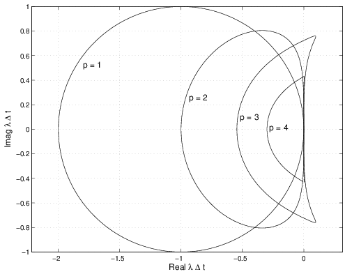
The stability boundary for these methods are shown in Figure 1.19. As the order of accuracy increases, the stability regions become smaller. Note, this is the opposite of Runge-Kutta methods for which the size of the stability regions increases with increased accuracy (see Section 1.9).