
2.5.1 Finite Volume Method in 1-D
Measurable Outcome 2.1, Measurable Outcome 2.3
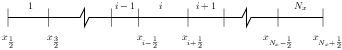
The basis of the finite volume method is the integral convervation law. The essential idea is to divide the domain into many control volumes and approximate the integral conservation law on each of the control volumes. For example, as shown in Figure 2.13, cell \(i\) lies between the points at \(x_{i-\frac{1}{2}}\) and \(x_{i+\frac{1}{2}}\). Note that the points do not have to be equally-spaced.
The one-dimensional form of Equation 2.1 is
Thus, applying this to control volume \(i\) (and recalling that \(S=0\) for convection) gives,
Next, we define the mean value of \(U\) in control volume \(i\) as,
Then, Equation 2.100 becomes,
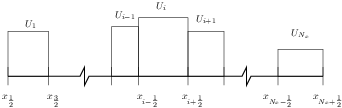
At this point, no approximations have been made thus Equation 2.102 is exact. Now, we make the first approximation. Specifically, we assume that the solution in each control volume is constant,
Thus, the finite volume approximation will be piecewise constant as shown in Figure 2.14.
With this assumed form of the solution, the next issue is to determine the flux at \(i\pm \frac{1}{2}\) at a time \(t\). This can be done with the knowledge that the solution convects with the velocity \(u(t)\). Thus, for the initial instant after \(t\) (which we denote as \(t^{+} = t + \epsilon\) where \(\epsilon\) is an infinitesimal, positive number):
The flux can be calculated directly from this value of \(U\),
An alternative way to write this flux which is valid regardless of the sign of \(u(t)\) is,
This flux, which uses the upstream value of \(U\) to determine the flux, is known as an ‘upwind' flux. When \(U\) is positive, the ‘upwind' direction is the negative \(x\) direction because the solution moves towards the positive \(x\) direction as \(t\) increases. When \(U\) is negative, the ‘upwind' direction is the positive \(x\) direction because the solution moves towards the negative \(x\) direction as \(t\) increases.
The final step in arriving at a full-discrete approximation for one-dimensional convection is to discretize Equation 2.102 in time. This can be done choosing any of the ODE integration methods we studied previously. For simplicity, we choose the forward Euler method so that the final fully-discrete form of the finite volume method is,
where we use the notation,