
1.7.1 Stiffness
Measurable Outcome 1.2, Measurable Outcome 1.9, Measurable Outcome 1.11, Measurable Outcome 1.12
Stiffness is a general (though somewhat fuzzy) term to describe systems of equations which exhibit phenoma at widely-varying scales. For the ODE's we have been studying, this means widely-varying timescales.
One way for stiffness to arise is through a difference in timescales between a forcing timescale and any characteristic timescales of the unforced system. For example, consider the following problem:
The forcing term oscillates with a frequency of \(1\). By comparison, the unforced problem decays very rapidly since the eigenvalue is \(\lambda =-1000\). Thus, the timescales are different by a factor of 1000.
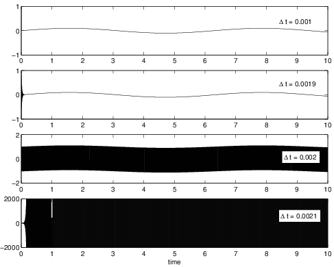
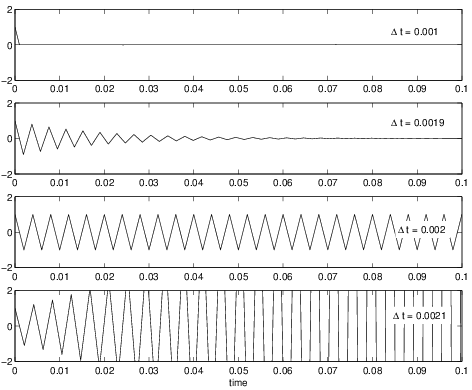
Suppose we are only interested in the long time behavior of \(u(t)\), not the initial transient. We would like to take a timestep that would be set by the requirements to resolve the \(\sin t\) forcing. For example, one might expect that setting \({\Delta t}= 2\pi /100\) (which would result in 100 timesteps per period of the forcing) would be sufficient to have reasonable accuracy. However, if the method does not have a large eigenvalue stability region, this may not be possible. In this case, the \({\Delta t}\) set by stability requirements is much smaller than what we need for accuracy. A small \({\Delta t}\) means that many iterations are needed, which makes the simulation computationally expensive. For example, if a forward Euler method is applied to this problem, eigenvalue stability would limit the \({\Delta t}\leq 0.002\) (since the eigenvalue is \(\lambda = -1000\) and the forward Euler stability region crosses the real axis at -2). The results from simulations for a variety of \({\Delta t}\) using forward Euler are shown in Figure 1.12. For \({\Delta t}= 0.001\), the solution is well behaved and looks realistic. For \({\Delta t}= 0.0019\), the approach of eigenvalue instability is evident as there are oscillations during the first few iterations which eventually decay. For \({\Delta t}= 0.002\), the oscillations no longer decay but remain throughout the entire simulation. Finally, for \({\Delta t}= 0.0021\), the oscillations grow unbounded. A zoomed image of these results concentrating on the initial time behavior is shown in Figure 1.13.
A more efficient approach to numerically integrating this stiff problem would be to use a method with eigenvalue stability for large negative real eigenvalues. Implicit methods often have excellent stability along the negative real axis. Recall from Lecture 3 that an implicit method is one in which the new value \(v^{n+1}\) is an implicit function of itself through the forcing function \(f\). The simplest implicit method is the backward Euler method,
The backward Euler method is first order accurate (\(p=1\)). The amplification factor for this method is,
When \(\lambda\) is negative real, then \(g < 1\) for all \({\Delta t}\). The eigenvalue stability region for the backward Euler method is shown in Figure 1.14.
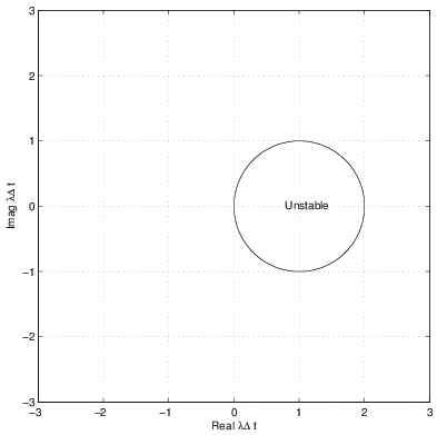
Only the small circular portion in the right-half plane is unstable while the entire left-half plane is stable. Results from the application of the backward Euler method to Equation 1.109 are shown in Figure 1.15.
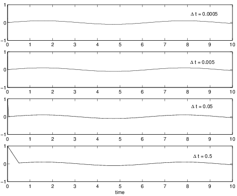
The excellent stability properties of this method are clearly seen as the solution looks acceptable for all of the tested \({\Delta t}\). Clearly, for the larger \({\Delta t}\), the initial transient is not accurately simulated, however, it does not effect the stability. Thus, as long as the initial transient is not desired, the backward Euler method will likely be a more effective solution strategy than the forward Euler method for this problem.
Another popular implicit method is trapezoidal integration,
Trapezoidal integration is second-order accurate (\(p=2\)). The amplification factor is,
The stability boundary for trapezoidal integration lies on the imaginary axis (see Figure 1.16).
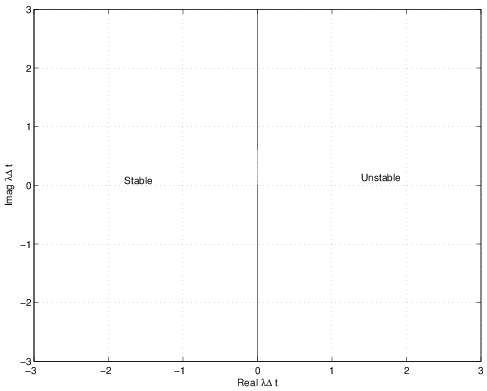
Again, this method is stable for the entire left-half plane thus it will work well for stiff problems.
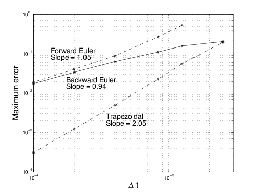
The accuracy of the forward Euler, backward Euler, and trapezoidal integration methods are compared in Figure 1.17 for Equation 1.109. The error is computed as the maximum across all timesteps of the difference between numerical and exact solutions,
These results show that the forward Euler method is first order accurate (since the slope on the log-log scaling is 1) once the \({\Delta t}\) is small enough to have eigenvalue stability (for \({\Delta t}> 0.002\) the algorithm is unstable and the errors are essentially unbounded). In contrast, the two implicit methods have reasonable errors for all \({\Delta t}\)'s. As the \({\Delta t}\) become small, the slope of the backward Euler and trapezoidal methods become essentially 1 and 2 (indicating first and second order accuracy). Clearly, if high accuracy is required, the trapezoidal method will require fewer timesteps to achieve this accuracy.
Stiffness from PDE discretization of diffusion problem
One of the more common ways for a stiff system of ODE's to arise is in the discretization of time-dependent partial differential equations (PDE's). For example, consider a one-dimensional heat diffusion problem that is modeled by the following PDE for the temperature, \(T\):
where \(\rho\), \(c_ p\), and \(k\) are the density, specific heat, and thermal conductivity of the material, respectively. Suppose the physical domain for of length \(L\) from \(x=0\) to \(x=L\). A finite difference approximation in \(x\) might divide the physical domain into a set of equally spaced nodes with distance \(h = L/(N-1)\) where \(N\) is the total number of nodes including the endpoints. So, node \(i\) would be located at \(x_ i = ih\). Then, at each node, \(T_{xx}\) is approximated using a finite difference derivative. For example, at node \(i\) we might use the following approximation,
Using this in the heat diffusion equation, we can find the time rate of change at node \(i\) as,
Thus, the \(T_ t\) at node \(i\) depends on the values of \(T\) at nodes \(i-1\), \(i\), and \(i+1\) in a linear manner. Since each node in the interior of the domain will satisfy the same equation, we can put the finite difference discretization of the heat diffusion problem into our standard system of ODE's form,
where \(A\) will be a tri-diagonal matrix (i.e. only the main diagonal and the two neighboring diagonals will be non-zero) since the finite difference approximation only depends on the neighboring nodes. The vector \(b\) will depend on the specific boundary conditions.
The question is how do the eigenvalues of \(A\) behave, in particular, as the node spacing \(h\) is decreased. To look at this, we arbitrarily choose,
since the magnitudes of these parameters will scale the magnitude of the eigenvalues of \(A\) by the same value but not alter the ratio of eigenvalues (the ratio is only altered by the choice of \(h/L\)). Figure 1.18 shows the locations of the eigenvalues for \(h/L = 0.1\) and \(h/L = 0.05\).
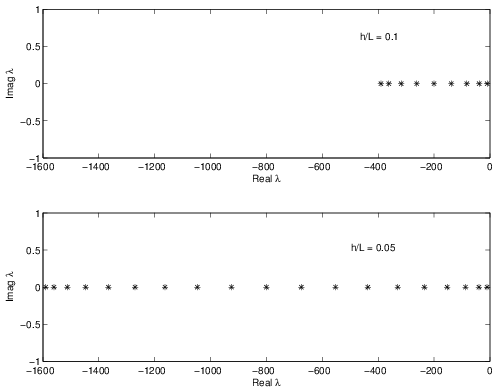
The eigenvalues are negative real numbers. The smallest magnitude eigenvalues appear to be nearly unchanged by the different values of \(h\). However, the largest magnitude eigenvalues appear to have increased by a factor of \(4\) from approximately \(-400\) to \(-1600\) when \(h\) decreased by a factor of \(2\). This suggests that the ratio of largest-to-smallest magnitude eigenvalues (i.e. the spectral condition number) is \(O(1/h^2)\).
The table above confirms this depends for a range of \(h/L\) values and also confirms that the smallest eigenvalue changes very little as \(h\) decreases.