2.3 Introduction to Finite Difference Methods

2.3.1 Finite Difference Approximations

Measurable Outcome 2.3, Measurable Outcome 2.6


Recall how the multi-step methods we developed for ODEs are based on a truncated Taylor series approximation for \(\frac{\partial U}{\partial t}\). Specifically, we can consider each multi-step method as computing \(U\) at discrete instances in time \((t^0, t^1, \ldots , t^ n, \ldots )\) where the derivative \(\left. \frac{\partial U}{\partial t}\right|_ n = U_ t^ n\) is approximated using a combination of \(\left(U^{n+1}, U^ n, U^{n-1}, \ldots \right)\).

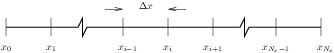
Finite difference methods for PDEs are essentially built on the same idea, but approximating spatial derivatives instead of time derivatives. Namely, the solution \(U\) is approximated at discrete instances in space \(\left(x_0, x_1, \ldots , x_{i-1}, x_ i, x_{i+1}, \ldots , x_{N_ x-1}, x_{N_ x}\right)\) where the spatial derivatives \(\left( \left.\frac{\partial U}{\partial x} \right|_ i = U_{x_ i}, \left. \frac{\partial ^2 U}{\partial x^2} \right|_ i = U_{xx_ i} \right)\) are approximated using a combination of \((U_ i, U_{i \pm 1}, U_{i \pm 2}, \ldots )\).

The figure shows a line of discrete instances in space with the span between each instance labeled as ”r.
Figure 2.8: One-dimensional structured mesh for finite difference approximations.


In the following we derive a finite difference approximation of \(\frac{\partial U}{\partial x}\) at node \(x_ i\). For a differentiable function \(U\), the derivative at the point \(x_ i\) is given by:

\[\left. \frac{\partial U}{\partial x} \right|_{x_ i} = \lim _{\Delta x \to 0} \frac{U(x_ i+\Delta x) - U(x_ i - \Delta x)}{2\Delta x}.\] (2.45)

The finite difference approximation is obtained by eliminating the limiting process:

\[{U_ x}_ i \approx \frac{U(x_ i+\Delta x) - U(x_ i-\Delta x)}{2 \Delta x} = \frac{U_{i+1} - U_{i-1}}{2 \Delta x} \equiv \delta _{2x} U_ i.\] (2.46)

The finite difference operator \(\delta _{2x}\) is called a central difference operator. Finite difference approximations can also be one-sided. For example, a backward difference approximation is,

\[\left.\frac{\partial U}{\partial x}\right|_{i,j} \approx \delta _{x}^{-} U_{i,j} \equiv \frac{1}{{\scriptstyle \Delta } x}\left(U_{i,j} - U_{i-1,j}\right), \label{equ:ux_ backwarddiff}\] (2.47)

and a forward difference approximation is,

\[\left.\frac{\partial U}{\partial x}\right|_{i,j} \approx \delta _{x}^{+} U_{i,j} \equiv \frac{1}{{\scriptstyle \Delta } x}\left(U_{i+1,j} - U_{i,j}\right), \label{equ:ux_ forwarddiff}\] (2.48)

We can also derive finite difference approximations for higher-order derivatives. For example, consider the following definition for the second derivative,

  \(\displaystyle \frac{\partial ^2 U}{\partial x^2}(x)\) \(\displaystyle =\) \(\displaystyle \lim _{{\scriptstyle \Delta } x\rightarrow 0} \frac{{\partial U}/{\partial x}(x+{\scriptstyle \Delta } x/2) - {\partial U}/{\partial x}(x-{\scriptstyle \Delta } x/2)}{{\scriptstyle \Delta } x}\)   (2.49)
    \(\displaystyle =\) \(\displaystyle \lim _{{\scriptstyle \Delta } x\rightarrow 0} \frac{1}{{\scriptstyle \Delta } x}\left[ \frac{U(x+{\scriptstyle \Delta } x)-U(x)}{{\scriptstyle \Delta } x} - \frac{U(x)-U(x-{\scriptstyle \Delta } x)}{{\scriptstyle \Delta } x}\right]\)   (2.50)
    \(\displaystyle =\) \(\displaystyle \lim _{{\scriptstyle \Delta } x\rightarrow 0} \frac{1}{{\scriptstyle \Delta } x^2}\left[ U(x+{\scriptstyle \Delta } x)-2U(x) + U(x-{\scriptstyle \Delta } x) \right].\)   (2.51)

The finite difference approximation for the second order derivative is obtained eliminating the limiting process.

\[\left.\frac{\partial ^2 U}{\partial x^2}\right|_{i,j} \approx \delta _{x}^2 U_{i,j} \equiv \frac{1}{{\scriptstyle \Delta } x^2}\left(U_{i+1,j} - 2 U_{i,j} + U_{i-1,j}\right). \label{equ:uxx_ centraldiff}\] (2.52)

Finite Difference Approximations in 2D

We can easily extend the concept of finite difference approximations to multiple spatial dimensions. In this case we represent the solution on a structured spatial mesh as shown in Figure 2.9.

The figure shows a grid with the first and second dimensions (perpendicular to each other), labeled similarly to Fig 2.8, with nodes at every intersection of the 2 dimensions.
Figure 2.9: Two-dimensional structured mesh for finite difference approximations.


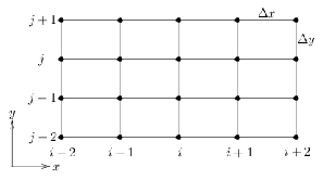
Using \(U_{i,j}\) to denote the value of \(U\) at node \((i,j)\) our central derivative approximations for the first derivatives are:

  \(\displaystyle \left.\dfrac {\partial U}{\partial x}\right|_{i,j}\) \(\displaystyle \approx\) \(\displaystyle \frac{U_{i+1,j} - U_{i-1,j}}{2 \Delta x} \equiv \delta _{2x} U_{i,j}.\)   (2.53)
  \(\displaystyle \left.\dfrac {\partial U}{\partial y}\right|_{i,j}\) \(\displaystyle \approx\) \(\displaystyle \frac{U_{i,j+1} - U_{i,j-1}}{2 \Delta y} \equiv \delta _{2y} U_{i,j}.\)   (2.54)

In general, finite difference approximations will involve a set of points surrounding \(U_{i,j}\).