
2.8.1 Functional Approximation of the Solution
In this lecture, we introduce the method of weighted residuals, which provides a general formulation for the finite element method. To begin, let's focus on the particular problem of steady heat diffusion in a rod. This problem can be modeled as a one-dimensional PDE for the temperature, \(T\):
where \(k(x)\) is the thermal conductivity of the material and \(f(x)\) is the heat source (per unit length). Note that both \(k\) and \(f\) could be functions of \(x\). Also, let the physical domain for the problem be from \(x=-L/2\) to \(x=L/2\).
Steady Heat Diffusion
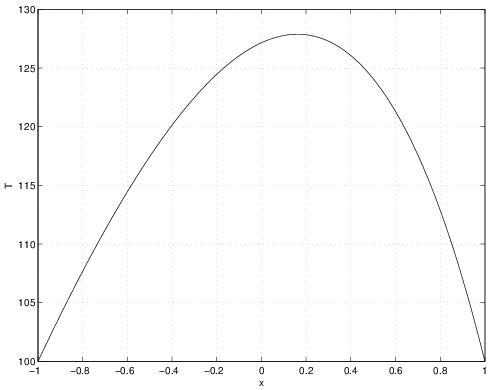
Suppose that the rod has a length of \(L=2\), the thermal conductivity is constant, \(k=1\), and the heat source is \(f(x) = 50 e^ x\). Assume that the temperature at the ends of the rod are to be maintained at \(T(\pm 1) = 100\). Equation (2.149) can be integrated twice to obtain:
Now, applying boundary conditions so that \(T(\pm 1) = 100\),
This is a \(2\times 2\) system which can be solved for \(a\) and \(b\) to find
where \(\cosh (y) = (e^ y + e^{-y})/2\) and \(\sinh (y) = (e^ y - e^{-y})/2\). Thus, the exact solution to this problem is
A plot of this solution is shown in Figure 2.25.
A common approach to approximating the solution to a PDE such as heat diffusion is to use a series of weighted functions. For example, for the temperature in the steady heat diffusion example we might assume that,
where \(\tilde{T}(x)\) is the approximation of \(T(x)\), \(N\) is the number of terms (functions) in the approximation, \(\phi _ j(x)\) are the (known) functions, and \(a_ j\) are the unknown function weights. The functions \(\phi _ j(x)\) are often called basis functions. They are usually designed to satisfy the boundary conditions. So, in this example where the temperature is 100 at \(x = \pm 1\), then \(\phi _ j(\pm 1) = 0\) (don't forget that \(\tilde{T}\) was defined to include the constant term of 100).
The question remains what functions (and how many) to choose for \(\phi _ j(x)\). While many good choices exist, we will use polynomials in \(x\) because polynomial approximations are used extensively in finite element methods (our main interest). For this problem, the following ideas can be used to determine the form of the \(\phi _ j(x)\):
-
First, we note that requiring \(\phi _ j(\pm 1) = 0\) places two conditions on each \(\phi _ j(x)\). These two conditions can be satisfied with a linear function of \(x\), but the linear function which equals 0 at \(x = \pm 1\) is simply \(0\). Since this does not add anything to the solution even after multiplying by a weight, the first non-trivial function would be a quadratic function.
-
A quadratic function can be designed to satisy the boundary conditions in the following manner,
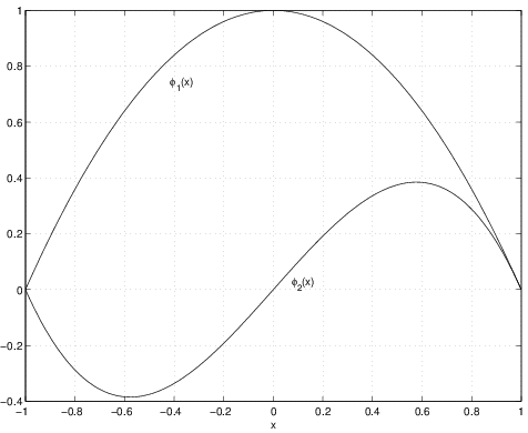
By including factors which go to zero at the end points, we have constructed a quadratic function which will satisfy the required boundary conditions. A plot of \(\phi _1(x)\) is shown in Figure 2.26.
-
Suppose we wanted to include a cubic polynomial in the approximation, then one way we could do this is multiply \(\phi _1(x)\) by \(x\).
Since \(\phi _1(x)\) goes to zero at the end points, then so will \(\phi _2(x)\). A plot of \(\phi _2(x)\) is shown in Figure 2.26. There are actually some better ways to choose these higher-order polynomials then simply multiplying the lowest order polynomial by powers of \(x\). The problem with the current approach is that if the number of terms were large (so that the powers of \(x\) would be large), then the set of polynomials (i.e., \(\phi _ j(x)\)) become very poorly conditioned resulting in many numerical difficulties. We will not discuss issues of conditioning but more advanced texts on finite element methods or related subjects can be consulted. For low order polynomial approximations, the issues of conditioning do not play an important role.
Figure 2.26: \(\phi _1(x)\) and \(\phi _2(x)\) for example heat diffusion problem.
Having selected a set of functions, we must now develop a way to determine values of \(a_ j\) that will lead to a good approximation of the actual \(T(x)\). While several ways exist to do this, we will focus on two methods in these introductory notes: the collocation method and the method of weighted residuals.