
3.3.2 Monte Carlo Analysis
Measurable Outcome 3.3, Measurable Outcome 3.5
In this lecture, we begin our exploration of probabilistic methods, i.e., numerical methods that are used to quantify the impact of uncertainty. In particular, we will focus on the Monte Carlo method, since it is the most common probabilistic analysis method and is the foundation for many others.
Why are probabilistic methods important for engineering analysis and design? More and more there is a realization of the importance of analyzing and managing uncertainty in engineering systems. There are many sources of uncertainty, including uncertain technology performance (especially for advanced technologies whose performance may not be proven in the field), variability due to manufacturing processes, uncertain operating conditions (e.g., weather conditions, wind gusts), and uncertainty due to limitations in the models we use. To be able to design robust, reliable, high-performance systems, we need to be able to analyze how all these different sources of uncertainty affect our system.
To make our discussion concrete, we will consider a simplified model for the heat transfer through a cooled turbine blade as shown in Figure 3.2.
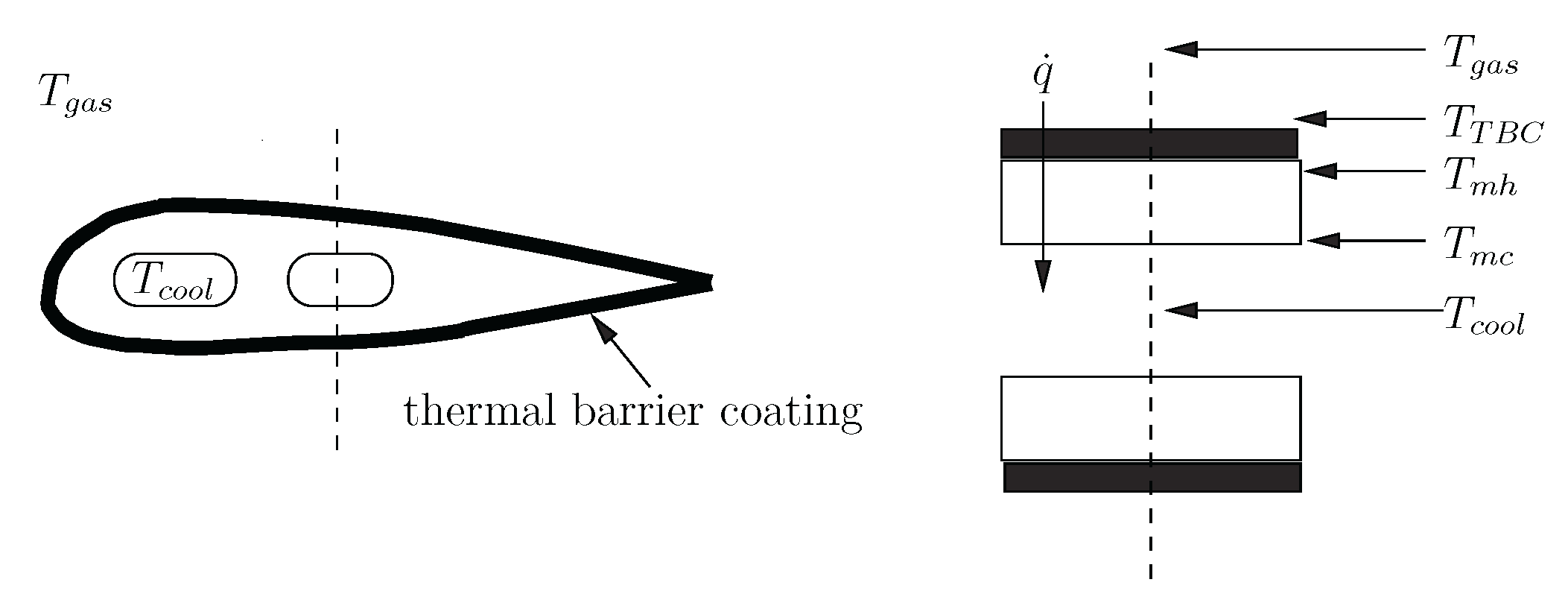
A one-dimensional model of the heat transfer along the dashed line is,
where \(h_{gas}\) and \(h_{cool}\) denote the convective heat transfer coefficients of the flow surrounding the blade and the cooling flow inside the blade, respectively. \(k_ m\) is the thermal conductivity of the metal and \(L_ m\) is the blade metal thickness. \(k_{TBC}\) is the thermal conductivity of the thermal barrier coating on the blade and \(L_{TBC}\) is the thickness of the thermal barrier coating. \(T\) denotes temperature, where the subscripts are \(_{gas}\) for the flow surrounding the blade, \(_{TBC}\) for the thermal barrier coating, \(_{mh}\) for the metal hot side, \(_{mc}\) for the metal cold side, and \(_{cool}\) for the cooling fluid.
Then, given the values of \(h_{gas}\), \(T_{gas}\), \(k_{TBC}\), \(L_{TBC}\), \(k_ m\), \(L_ m\), \(h_{cool}\), and \(T_{cool}\), we can solve these four equations to determine, \(T_{TBC}\), \(T_{mh}\), \(T_{mc}\), and \(\dot{q}\). In the design of cooled turbine blades, a key measure of system performance is the hot-side metal temperature, \(T_{mh}\), because as this temperature increases, the durability (usable life) of a blade decreases. Thus, the goal of the heat transfer design is to maintain the metal temperatures at an acceptably low value while minimizing cost.
Nominal Analysis of Turbine Blade Heat Transfer
A typical, deterministic analysis of the turbine blade heat transfer problem would assume that all of the input parameters are at their nominal (i.e., design-intent) values. Suppose the design-intent values were,
The results of this design-intent analysis give,
Analysis of Turbine Blade Heat Transfer Under Uncertainty
Due to manufacturing variability, the parameters of the actual manufactured blades are not exactly the design-intent values but rather are distributed over a range of values. For example, due to the difficulty of applying the thermal barrier coating on the outside of the blades, the thickness of the thermal barrier coating is variable.
The role of probabilistic methods is to quantify the impact of this type of variability on properties of interest (e.g., the hot-side metal temperature). The results of the probabilistic analysis can take many forms depending on the specific application. In the example of the turbine blade where the hot-side metal temperature is critical, the following information might be desired from a probabilistic analysis:
-
The distribution of \(T_{mh}\) that would be observed in the population of manufactured blades.
-
The probability that \(T_{mh}\) is above some critical value (indicating the blade's life will be unacceptably low).
-
Instead of determining the entire distribution of \(T_{mh}\), sometimes knowing the mean value, \(\mu _{T_{mh}}\), is sufficient.
-
To have some indication of the variability of \(T_{mh}\) without requiring accurate estimation of the entire distribution, the standard deviation, \(\sigma _{T_{mh}}\), can be used.
The Monte Carlo method is based on the idea of taking a small, randomly-drawn sample from a population and estimating the desired outputs from this sample. For the outputs described above, this would involve:
-
Replacing the distribution of \(T_{mh}\) that would be observed over the entire population of manufactured blades with the distribution (i.e., histogram) of \(T_{mh}\) observed in the random sample.
-
Replacing the probability that \(T_{mh}\) is above a critical value for the entire population of manufactured blades with the fraction of blades in the random sample that have Tmh greater than the critical value.
-
Replacing the mean value of \(T_{mh}\) for the entire population with the mean value of the random sample.
-
Replacing the standard deviation of \(T_{mh}\) for the entire population with the standard deviation of the random sample.
In Summary
In the next unit, we will see how to carry out this analysis using Monte Carlo simulation. In summary, our probabilistic analysis involves three steps:
-
Generate a random sample of the input parameters according to the (assumed) distributions of the inputs.
-
Analyze (deterministically) each set of inputs in the sample.
-
Estimate the desired probabilistic outputs (e.g., mean, standard deviation), and the uncertainty in these outputs, using the random sample.